smhuang2006_scu
smhuang2006
Recently Published


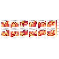
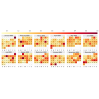
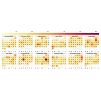
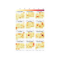
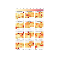
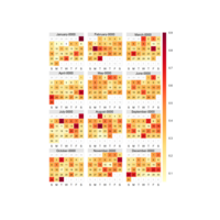
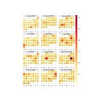
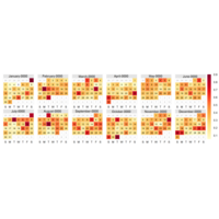
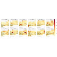
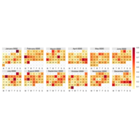
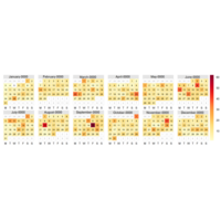
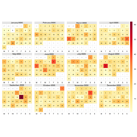
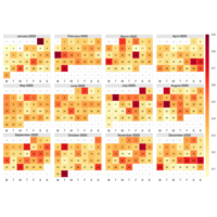
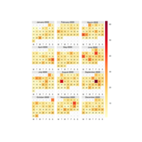
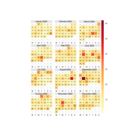
Plot. calendar heatmap
calendar heatmap

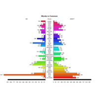
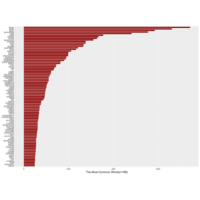
Plot. A plorized tag plot
two books
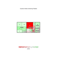
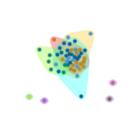
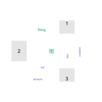
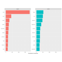
Plot (treemap, Kwartler, 2017:169)
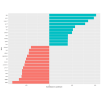
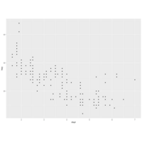
Figure 5.21 Illustrating the articles’ size, polarity and topic grouping.

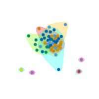
Plot(Polarity, Kwartler, 2017: 169)
Figure 5.21 Illustrating the articles’ size, polarity and topic grouping.
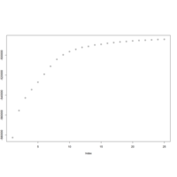
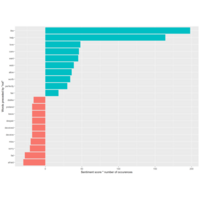
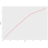
Plot (log likelihoods plot, Kwartler, 2017: 164)
Figure 5.19 The log likelihoods from the 25 sample iterations, showing it improving and
then leveling off.
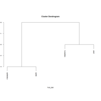
Plot (cluster dendrogram, Kwartler, 2017: 154)
Figure 5.17 The example fruit dendrogram.
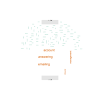
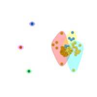
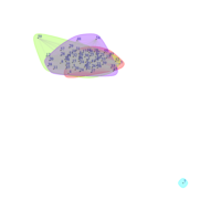
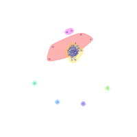
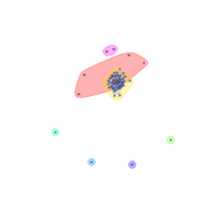
Plot (Medoid comparison cloud, Kwartler, 2017: 147)
Figure 5.15 Mediod prototype work experiences 15 & 40 as a comparison cloud.
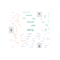
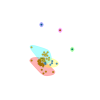
Plot (Spherical k-means comparison cloud, Kwartler, 2017: 143)
Figure 5.13 The spherical k‐means comparison cloud improves on the original in the
previous section.
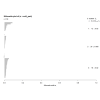
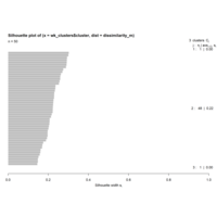
Plot (spherical k‐means silhouette plot, Kwartler, 2017: 142)
Figure 5.12 The spherical k‐means silhouette plot with three distinct clusters.
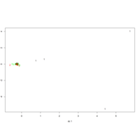
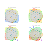
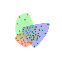
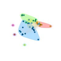
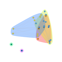
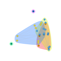
Plot (spherical k-means cluster plot, Kwartler, 2017: 142)
Figure 5.11 The spherical k‐means cluster plot with some improved document separation.
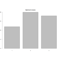
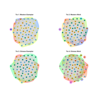
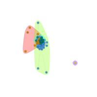
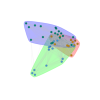
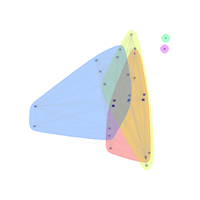
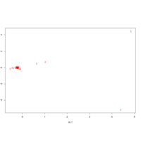
Plot (Figure 5.10, spherical k-means, Kwartler, 2017: 141)
Figure 5.10 The cluster assignments for the 50 work experiences using spherical k‐means.
Plot (Figure 5.8, Kwartler, 2017: 138)
Figure 5.8 The comparison clouds based on
prototype scores.
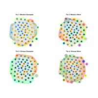
我的图与书上的很不一样啊?
Plot (Figure 5.7, Kwartler, 2017: 137)
Figure 5.7 The k‐means clustering silhouette plot dominated by a single cluster.
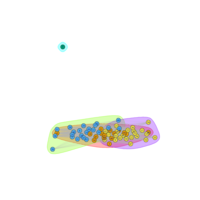
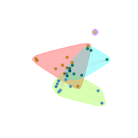
Plot (Figure 5.6, Kwartler, 2017: 136)
Figure 5.6 The plotcluster visual is overwhelmed by the second cluster and shows
that partitioning was not effective.
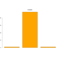
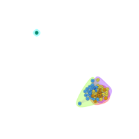
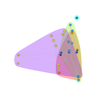
Plot (Figure 5.5, Kwartler, 2017: 136)
Figure 5.5 The k‐means clustering with three partitions on work experiences.
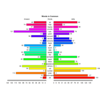
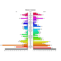
Plot (Figure 3.17, pyramid plot, Kwartler, 2017: 82)
Figure 3.17 An example polarized tag plot showing words in common between corpora. R will plot a larger version for easier viewing.
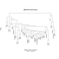
Plot (a dendrogram, Kwartler, 2017, p.70)
Figure 3.10 A reduced term DTM, expressed as a dendrogram for the @DeltaAssist corpus.
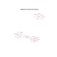
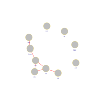
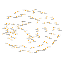
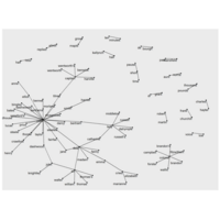
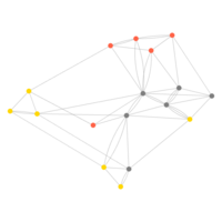
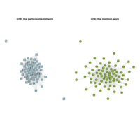
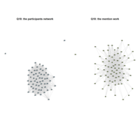
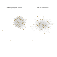
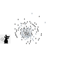
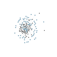
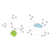
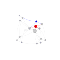
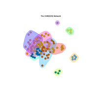
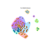
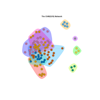
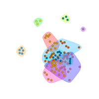
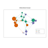
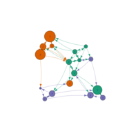
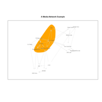
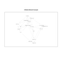
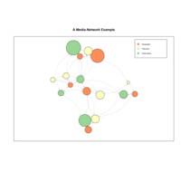
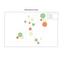
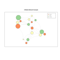
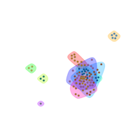
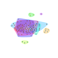
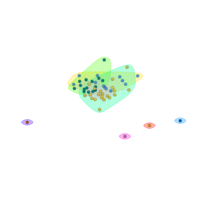
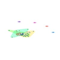
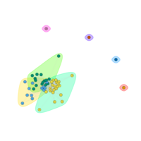
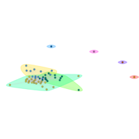
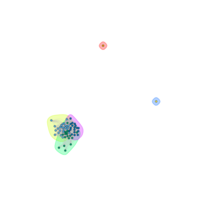
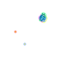
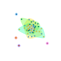
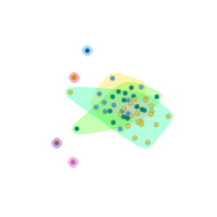
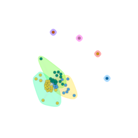
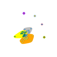
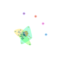
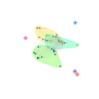
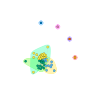
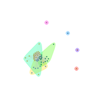
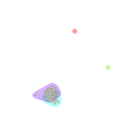
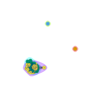
Plot (A Word Network, Figure 3.6, Kwartler, 2017: 64)
Figure 3.6 A very small word network using the igraph package.
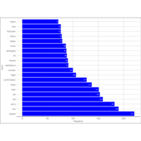
Plot (Figure 3.1, Kwartler, 2017: 56)
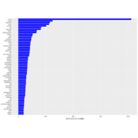
Figure 3.1 The bar plot of individual words has expected words like please, sorry and flight
confirmation.
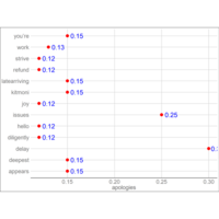
Plot. Figure 3.2 (Kwartler,2017,p.58)
Figure 3.2 Showing that the most associated word from DeltaAssist’s use of apologies
is “delay”
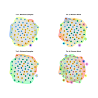
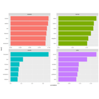
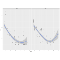
Plot
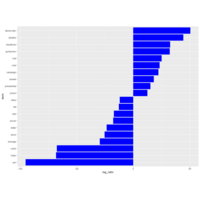
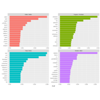
beta差异最大的词(Text Mining with R, Silge & Robinson,中文,p89)
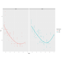
Plot
LDA双主题(图6-2,Text Mining with R, Silge & Robinson,中文,p.88)
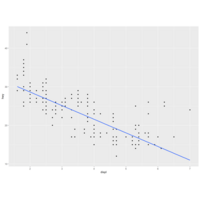
Plot (my exercise)
2020-06-06
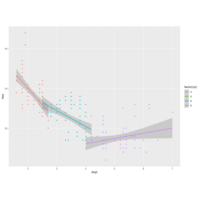
Plot
AP articles (Text Mining with R, Silge & Robinson,中文,p.71)
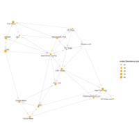
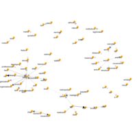
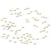
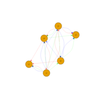
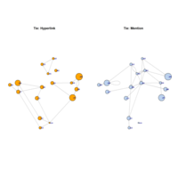
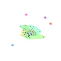
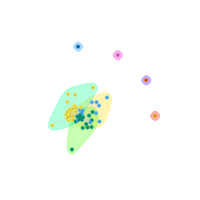
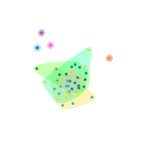
Plot
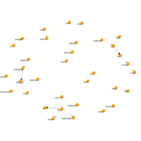
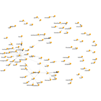
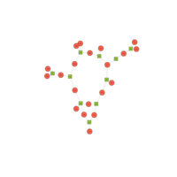
相关性大于0.15的单词对的网络图(Text Mining with R,Silge & Robinson,中文,p.66)
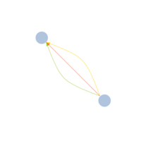
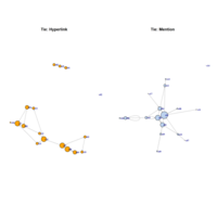
Plot
图4-8(Text Mining with R, Silge & Robinson,中文,p.65)
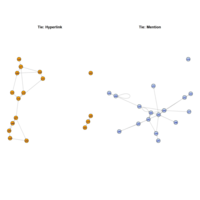
Plot
圣经二元组网络图(Text Mining with R, Silge & Robinson,中文,p.60)
Plot
二元组网络图(未润色,Text Mining with R, Silge & Robinson,中文,p.57)
Plot
二元组网络图(润色,Text Mining with R,中文,p.58)
Plot
“not”后的单词(Text Mining with R, Silge & Robinson,p.53)
Plot
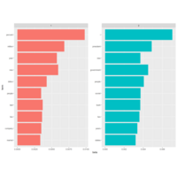
物理学文本tf-idf(Text Mining with R, Silge & Robinson,中文,p.42)
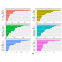
Plot
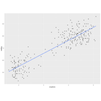
tf_idf (Text Mining with R, Silge & Robinson,中文,p.40)
Plot
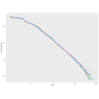
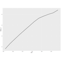
Zipf law index (Text Mining with R,中文,p.38)
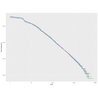
Plot
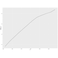
Text Mining with R (Silge & Robinson,中文,p.37)
Plot
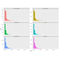
Text Mining with R (Silge & Robinson,中文,p.35)
Plot
Text Mining with R (Silge & Robinson,中文,p.27)
Plot
Text Mining with R (Silge & Robinson,中文,p.25)
Plot
Text Mining with R (Silge & Robinson, 中文,p.23)


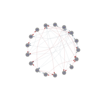
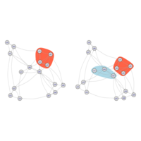
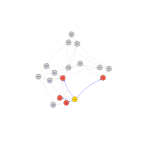
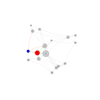
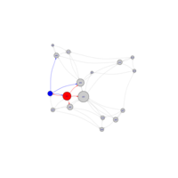
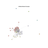

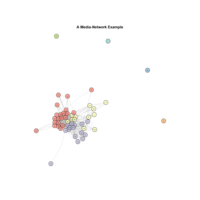
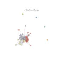
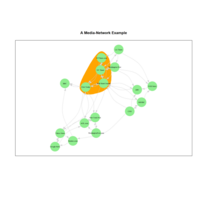

learn how to plot in igraph
modularity
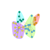
学习community detection
multilevel